CASPULE — Setup • Simulate • Analyze Sticker–Spacer Polymers
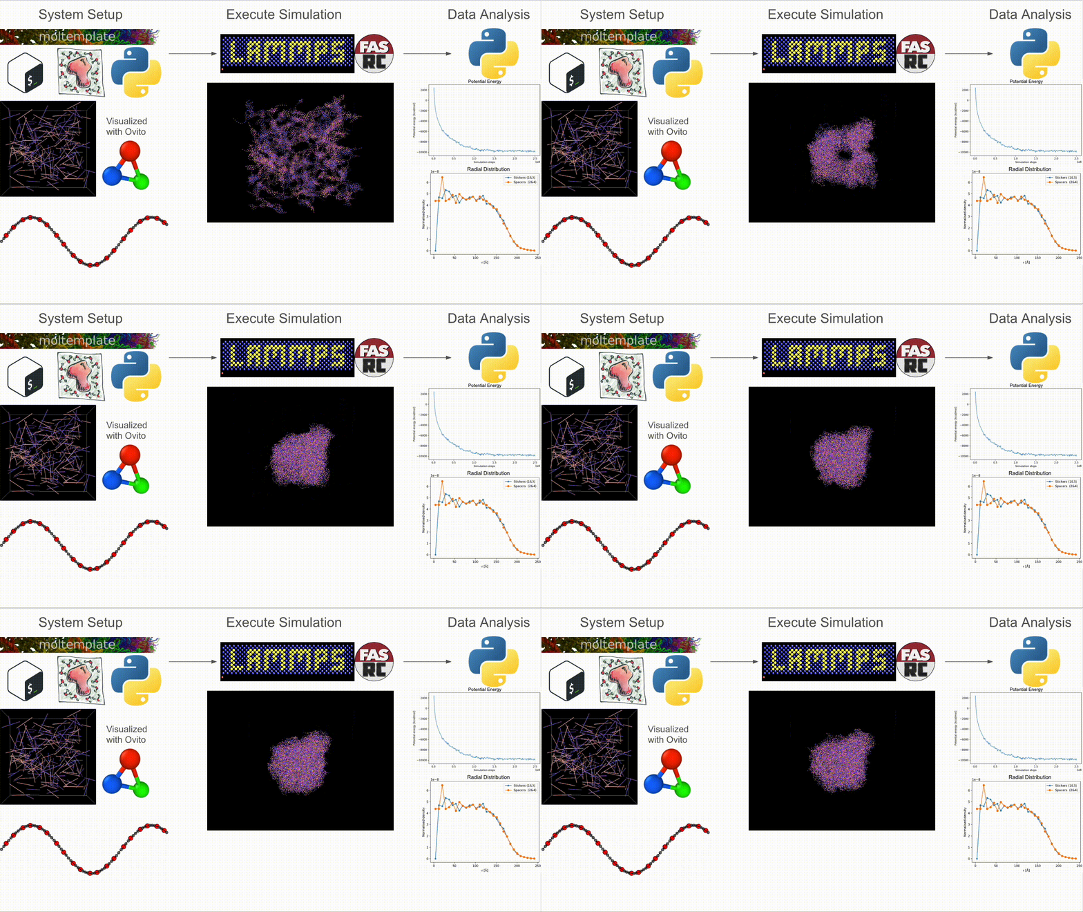
CASPULE, (C)ondensate (A)nalysis of (S)ticker Spacer (P)olymers (U)sing the (L)AMMPS (E)ngine, is a pipeline for Langevin Dynamics simulations of coarse-grained biopolymers. It automates system setup, LAMMPS simulation, and analysis of sticker–spacer polymer phase behavior. It provides an end-to-end reproducible computational protocol to simulate and analyze biological condensates.
Overview
CASPULE is a three-stage pipeline for simulations of sticker–spacer polymers:
Step 1 — Setup: Build arbitrary lengths and patterns; generate Packmol + Moltemplate inputs and a LAMMPS-ready
*.data(initial condition).Step 2 — Simulate: Run Langevin dynamics (with optional metadynamics via Colvars) in LAMMPS; supports MPI + load balancing.
Step 3 — Analyze: Turn trajectories/restarts into cluster statistics, bonded-sticker fractions, radial profiles, and energy timecourses.

Why CASPULE?
Arbitrary patterns & lengths: Repeatable block templates let you sweep architectures systematically.
Saturating interaction: Single-valent sticker interaction (to mimic saturable biomolecular interactions) and tunable
E_svsE_ns.Batteries-included analysis: Reproducible Python tools for kinetics and steady-state structure.
Quick Start (End-to-End)
Prerequisites
Ensure these are on $PATH (or module-loaded):
LAMMPS with
fix bond/create/random,bond/break, Colvars (for metadynamics), MPI build recommendedPython 3 with the packages listed in Installation
Step 1 — Setup (build data + inputs)
Run the setup wrapper; it orchestrates all sub-steps.
bash create_InitCoor.sh
Behind the scenes, CASPULE executes:
python3 LT_writer.py <n> <seg_pattern>(make block templates)python3 writePackmolInput.py <n> <NA> <NB> <L> populate_tmp.inp IC_tmp.xyzpython3 writeSysLT.py <n> <NA> <NB> <L> b70_N200_L<L>.ltpackmol < populate_tmp.inpmoltemplate.sh -xyz IC_tmp.xyz b70_N200_L<L>.lt -nocheckpython3 updateColVar.py IC_tmp.xyz N200_Rg_L<L>.colvars <L> <n> <NA> <NB> <seg_pattern>python3 updateInput.py Template_input.in <L>python3 fix_datafiles.py b70_N200_L<L>.data
Artifacts produced:
IC_tmp.xyz
polyA_n<n>.lt, polyB_n<n>.lt
b70_N200_L<L>.lt
b70_N200_L<L>.data
b70_N200_L<L>.in
N200_Rg_L<L>.colvars
submit_b70_N200_L<L>.sh
Step 2 — Simulate (Langevin ± Metadynamics)
Vanilla Langevin:
mpirun -np 40 lmp -in b70_N200_L<L>.in
Notes
Specific interaction
Single-valent stickers via fix bond/create/random + bond/break,
with shifted-harmonic bonds (well depth E_s).
Non-specific interaction
LJ (pair_style lj/cut) with well depth E_ns;
LJ interactions between bonded beads are excluded (special_bonds lj 0 1 1 angle yes).
Typical parameter choices
- r0 = 1.122 σ with σ = 10 Å
- r_cut = r0 + 1.5 Å
- T = 310 K
- timestep 20–30 fs
- tdamp ≈ 500 fs
Parallel scaling rule of thumb
~500 beads / CPU; enable simulation load balancing for spatially heterogenous systems
(comm_style tiled + fix balance).
Metadynamics (optional): supply Colvars (e.g., N200_Rg_L<L>.colvars) to accelerate process of interest (clustering, coalescence etc.) along user defined collective variables (Rg, Inter-cluster distance etc.).
Step 3 — Analyze (one-command reports)
Use the analysis scripts in Data-Analysis Helpers to compute:
Cluster size distributions (graph-based from
*.restart)Bonded-sticker fraction vs time
Radial density profiles (stickers vs spacers)
Potential energy timecourses (convergence diagnostics)
Example:
python3 analysis/cluster_size_distribution.py   /path/to/sim_folder
python3 analysis/bonded_sticker_fraction.py     /path/to/Thermo_*.dat
python3 analysis/radial_profiles.py             /path/to/restarts
Get Started / Learn More
Contents:
- Installation
- Model Overview
- Pipeline Overview
- Example System Setup
- Simulation Output
- Thermodynamic Data:
Thermo_<fName>.dat - Bond-Formation/Breaking Data:
BondData_<fName>.dat - Collective-Variable Trajectory:
<fName>.colvars.traj - LAMMPS Dump Trajectory:
traj_<fName>.dump - Colvars Metadynamics Hills:
<fName>.colvars.meta-radgy.hills.traj - Potential of Mean Force (PMF):
<fName>.pmf - Restart Files
- LAMMPS Log File:
<fName>.log - Summary of All Simulation Outputs
- Thermodynamic Data:
- Data-Analysis Helpers
- Potential-Energy Trace
- Bonded-Sticker Fraction (BSF) – time series
- Cluster Size vs Bound-Sticker Fraction (scatter)
- Sticker Dissociation Events
- Cluster-Size Distribution
- Radial Sticker / Spacer Density
- Chain-Neighbour Histogram
- Sticker-Bond Multiplicity per Chain Pair
- Inter-molecular Sticker‑Sticker Distances
- API Reference
Contributing & Issues
Please open issues or PRs on the repository. Include your LAMMPS version/tag and whether Colvars + bond/create/random are enabled.